k-Means Clustering Tutorial in RapidMiner

In this tutorial, I will attempt to demonstrate how to use the k-Means clustering method in RapidMiner. The dataset I am using is contained in the Zip_Jobs folder (contains multiple files) used for our March 5^th Big Data lecture.

•  Save the files you want to use in a folder on your computer.
• Open RapidMiner and click “New Process”. On the left hand pane of your screen, there should be a tab that says "Operators"- this is where you can search and find all of the operators for RapidMiner and its extensions. By searching the Operators tab for "process documents", you should get an output like this (you can double click on the images below to enlarge them):

You should see several Process Documents operators, but the one that I will use for this tutorial is the “Process Documents from Files” operator because it allows you to generate word vectors stored in multiple files. Drag this operator into the Main Process frame.

• Click “Edit List” beside the “text directories” label in the right-hand pane in order to choose the files that you wish to run the clustering algorithm on.

You can choose whatever name you wish to name your directory.

Click the folder icon to select the folder that contains your data files. Click “Apply Changes”.

• Double click the “Process Documents from Files” operator to get inside the operator. This is where you will link operators together to take the (in my case) html documents and split them down into their word components (please note that you can run the K-Means Clustering algorithm with a different type of file). As highlighted in my previous tutorial, there are several operators designed specifically to break down text documents. Before you get to that point, you need to strip the html code out of the documents in order to get to their word components. Insert the “Extract Content” operator into the Main Process frame by searching for it in the Operators tab.

• The next thing that you would want to do to your files is to tokenize it. Tokenization creates a "bag of words" that are contained in your documents. Search for the "Tokenize" operator and drag it into the "Process Documents from Files" process after the “Extract Content” operator. The only other operator that is necessary to include for appropriate clustering for documents is the “Transform Cases” operator; without this, documents that have the same words in different cases would not be considered as more distant (less similar) documents. You should get a process similar to this: 

• Now for the clustering! Click out of the “Process Documents from Files” process. Search for “Clustering” in the Operators Tab:

As you can see, there are several clustering operators and most of them work about the same. For this tutorial, I chose to demonstrate K-Means clustering since that is the clustering type that we have discussed most in class. In RapidMiner, you have the option to choose three different variants of the K-Means clustering operator. The first one is the standard K-Means, in which similarity between objects is based on a measure of the distance between them. The K-Means (Kernel) operator uses kernels to estimate the distance between objects and clusters. The k-Means (fast) operator uses the Triangle Inequality to accelerate the k-Means algorithm. For this example, use the standard k-Means algorithm by dragging into the Main Process frame after the “Process Documents from Files” operator. I set the k value equal to 4 (since I have 19 files, this should give me roughly 5 files in each cluster) and max runs to about 20.

• Connect the output nodes from the “Clustering” operator to the res nodes of the Main Process frame. Click the “Play” button at the top to run. Your ExampleSet output should look like this:

 By clicking the folder view under the “Cluster Model” of the output, you can see which documents got placed into each cluster.

If you do not get this output, make sure that all of your nodes are connected correctly and also to the right type. Some errors are because your output at one node does not match the type expected at the input of the next node of an operator. If you are still having trouble, please comment or check out the Rapid-i support forum.

A tip for using trained models in RapidMiner

There are some cases that you may train a model like Artificial Neural Network, SVD or Linear regression in RapidMiner and you may need to reapply your model to the other testing data in future. There are two options to handle it. The first option is to save the model for future use and reopen it when it is needed and then update the old test data set with the newer data set and run the model. This option is reasonable when the training process does not last so long. In the cases that you are dealing with a huge data set and your model needs couple of hours to get trained, like ANN models, this option seems tedious. The second way to handle this problem is to just save the trained model and then apply it later on the new data set. In this post I will illustrate this process.

At first you need to build the original model. Let’s say that we have an ANN model similar to the following figure.

 To save the trained model, you should use Write Model operator. Search for this operator and add it to the model and connect the mod port of the Neural Net operator to the mod port of the Write Model operator and then connect the thr port to the mod port of the Apply Model as illustrated in the figure below. In your computer create a new Text file. It will be used by RapidMiner to save the model. Afterward, in Write Model operator properties window enter the address of the new created text file in model file textbox.

You can also add the Write Model operator after the Apply Model operator too, like the following figure.

Now, when you are going to test your model on the new test data set, you need to create a new project and then import your saved model to this process by using Read Model operator. Add the Apply Model operator and then import the new data set to the model and connect it to the unl port of the Apply Model operator. Your model should look like the following operator.

Linear Regression in RapidMiner

Regression models are useful and understandable models which are used for prediction and data fitting. RapidMiner provides simple tool for regression which I am going to illustrate how to use it in this post.

The first step is to import the training data by using appropriate Read operator. Then you may change the attribute type of your target field (dependent variable) to label by using Set Role operator. Adding the Linear Regression operator, your model should look like the figure below.

The min tolerance property of Linear Regression operator is confidence level or alpha level in statistic language. Now, you can import your test data and use the Apply Model operator to predict the data. Your model should look like the following figure.

If you connect the weight port of the Linear Regression operator to the result port of process windows, you can see the weights of independent variables in the separate table. I ran my model which contains 5 independent variables and one dependent variable. the following graphs show the results. RapidMiner provides you with the statistics result related to the regression model and the equation and adds a prediction field to the test data set. You can export the results to the excel by using write to Excel operator

Decision Tree in RapidMiner

Decision Trees are useful techniques for classification, prediction and fitting data. In this post I demonstrate how to build a basic decision tree model in RapidMiner.

At first you need to make sure that your data only contains attribute and label types which are allowed in Decision Tree operator. As you can see in the below figure, the Decision Tree operator just accepts Polynomial, Numerical and Binomial attributes and Binomial and Polynomial labels (target attributes). So, if your target data is a numeric variable you may modify it to the accepted type by categorizing it into several intervals and then defining dummy binomial attributes for each interval. I explained this process in my previous post.

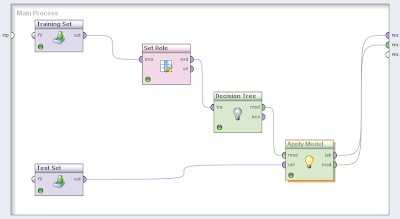
Once you prepared your data based on the allowable attributes and labels, you are ready to build the model. Add a Read Excel operator and import your training data set to this operator and then use a Set Role operator to set the target attribute role to Label and then add a Decision Tree operator. Connect these operators to each other in the order that you added them to the model. Your model should looks like the figure below.

Now add the second Read Excel operator to import the test data set. then add the Apply Model operator and connect its unlabeled port to the out port of the Read Excel operator for the test data and its model port to the model port of the Decision Tree operator as illustrated in the figure below.

The Apply model does not accept the data set which has the label attribute. So if the test data set contains the target attribute, you should eliminate this attribute and let the RapidMiner to fill out it by itself. As an example, I built a model based on a data set which contains 5 numeric regular attributes and a target binomial label which has two values Min and Max. The following figures show the results.

As you see, RapidMiner has created three attributes which are distinguished by pink color in Meta Data View window. Because my target label has two possible outputs, RapidMiner created an attribute for every outputs and calculated their occurrence probabilities for all instances. In the third created attribute, RapidMiner predicts the output for each instance based on the output probabilities. The output with the highest probability is the most likely occurring event, so it is reported as a prediction for that instance. Furthermore in the tab Tree, you can see the generated decision tree for your problem and analyze it.

In my model, “3hr sum” and “month sum” attributes are the most affecting attributes in the model, respectively. In the Text view, you can see the tree summary and also the branches confidences.

Install Rapidminer in Linux (ubuntu)

Installing rapid miner in Linux is a little bit different than it in Windows. Also according to the descriptions of official website, this method could be used any platform. (My Linux distr is Ubuntu 12.04)

The first step is to install java. Open terminal first, and enter and execute these commands one by one. 

sudo apt-get purge openjdk*

sudo add-apt-repository ppa:webupd8team/java

sudo apt-get update

sudo apt-get install oracle-java7-installer

In the installing process, the system will ask whether to continue, please just enter "y" to continue. 

After java is installed, download Rapidminer  form the its website. Please choose the right version shwon in picture below. Usually, they could detect the system automatically, if not, please choose the proper one, and download. 

After download, choose a destination folder to unzip the downloaded file. I extracted it in the "download" folder. 

After step, please click the extracted folder, and find the file named "rapidminer.jar"

Please do not double click it to open directly. Right click this file--> "open with oracle java 7 runtime", then rapid miner will be ran. Then interface is as same as it in other os. 

Ref: http://www.ubuntugeek.com/how-to-install-oracle-java-7-in-ubuntu-12-04.html

        http://rapid-i.com

Video Tutorial: A tip to enhance RapidMiner performance

In this video, I show you how to arrange the running order of parallel process in RapidMiner so that the computer memory is allocated to the operators efficiently.

Video Tutorial: Neural Network Toolbox in MATLAB

Following my previous video about building Neural Network model in RapidMiner, I made an introductory video to show how to work with Neural Network Toolbox in MATLAB.

Text Processing Tutorial with RapidMiner

     I know that a while back it was requested (on either Piazza or in class, can't remember) that someone post a tutorial about how to process a text document in RapidMiner and no one posted back. In this tutorial, I will try to fulfill that request by showing how to tokenize and filter a document into its different words and then do a word count for each word in a text document (I am essentially showing how to do the same assignment in HW 2 (plus filtering) but through RapidMiner and not AWS).

1) I first downloaded my document (The Entire Works of Mark Twain) through Project Gutenberg's website as a text document. Save the document in a file on your computer.

2) Open RapidMiner and click "New Process". On the left hand pane of your screen, there should be a tab that says "Operators"- this is where you can search and find all of the operators for RapidMiner and its extensions. By searching the Operators tab for "read", you should get an output like this (you can double click on the images below to enlarge them):

There are multiple read operators depending on which file you have, and most of them work the same way. If you scroll down, there is a "Read Documents" operator. Select this operator and enter it into your Main Process window by dragging it. When you select the Read Documents operator in the Main Process window, you should see a file uploader in the right-hand pane. 

 Select the text file you want to use.

 3) After you have chosen your file, make sure that the output port on the Read Documents operator is connected to the "res" node in your Main Process. Click the "play" button to check that your file has been received correctly. Switch to the results perspective by clicking the icon that looks like a display chart above the "Process" tab at the top of the Main Process pane. Click the "Document (Read Document)" tab. Your output text should look something like this depending on the file you have chosen to process:

4) Now we will move on to processing the document to get a list of its different words and their individual count. Search the Operators list for "Process Documents". Drag this operator the same way as you did for the "Read Documents" operator into the main pane.

Double click the Process Documents operator to get inside the operator. This is where we will link operators together to take the entire text document and split it down into its word components. This consists of several operators that can be chosen by going into the Operator pane and looking at the Text Processing folder. You should see several more folders such as "Tokenization", "Extraction", "Filtering", "Stemming", "Transformation", and "Utility". These are some of the descriptions of what you can do to your document.  The first thing that you would want to do to your document is to tokenize it. Tokenization creates a "bag of words" that are contained in your document. This allows you to do further filtering on your document. Search for the "Tokenize" operator and drag it into the "Process Documents" process. 

Connect the "doc" node of the process to the "doc" input node of the operator if it has not automatically connected already. Now we are ready to filter the bag of words. In "Filtering" folder under the "Text Processing" operator folder, you can see the various filtering methods that you can apply to your process. For this example, I want to filter certain words out of my document that don't really have any meaning to the document itself (such as the words a, and, the, as, of, etc.); therefore, I will drag the "Filter Stopwords (English)" into my process because my document is in English. Also, I want to filter out any remaining words that are less than three characters. Select "Filter Tokens by Length" and set your parameters as desired (in this case, I want my min number of characters to be 3, and my max number of characters to be an arbitrarily large number since I don't care about an upper bound). Connect the nodes of each subsequent operator accordingly as in the picture.

 After I filtered the bag of words by stopwords and length, I want to transform all of my words to lowercase since the same word would be counted differently if it was in uppercase vs. lowercase. Select the operator "Transform Cases" and drag it into the process.

 5) Now that I have the sufficient operators in my process for this example, I check all of my node connections and click the "Play" button to run my process. If all goes well, your output should look like this in the results view:

 Congrats! You are now able to see a word list containing all the different words in your document and their occurrence count next to it in the "Total Occurences" column. If you do not get this output, make sure that all of your nodes are connected correctly and also to the right type. Some errors are because your output at one node does not match the type expected at the input of the next node of an operator. If you are still having trouble, please comment or check out the Rapid-i support forum.

Video Tutorial: Neural Network in RapidMiner

This tutorial shows how to build a Neural Network model in RapidMiner.

Support Vector Machines with RapidMiner

The support vector machine (SVM) approach represents a data-driven method for solving classification tasks. It has been shown to produce lower prediction error compared to classifiers based on other methods like artificial neural networks, especially when large numbers of features are considered for sample description.


1 Introduction

Support Vector Machines (SVMs) are a technique for supervised machine learning. They can perform classification tasks by identifying hyperplane boundaries between sets of classes. The original linear SVMs were developed by Vapnik and Lerner (1963) and were enhanced by Boser, Guyon, and Vapnik (1992) to be applied to non-linear datasets.

2 Linear models
In the case of linearly separable classes, a maximum margin hyperplane is constructed such that the boundary line stays as far away as possible from each class, as shown in Figure 1a.
The hyperplane is constructed by constructing a linear function:

Each instance has i attributes that define it. The weights, w, are calculated during the training step to build
the linear function. One method of iteratively calculating the weights is the perceptron method.

In the case that the two classes are not linearly separable, the soft margin optimisation can be performed (Figure 1b). If instances fall on the “wrong” side of the maximum margin hyperplane, the distance between the instance and the maximum margin hyperplane, known as the slack is minimised.

In addition to classifying tasks, linear models can be used for regression. Least squares regression can be used to fit a line to a dataset and new numerical values can be predicted for new instances. This technique can also be extended into non-linear space in a similar manner to the non-linear modeling process.

3 Support vectors
Support vectors are instances that are the closest to the linear boundary. There is always at least one support vector per class, often there are more. The support vectors can be chosen by constrained quadratic optimisation. The maximum margin hyperplane can be created using just the support vectors. This means that identifying the support vectors and removing all other instances before creating the linear model results in a computationally cheaper process.
In addition, choosing support vectors reduces the possibility of overfitting the training data. This is because the only time the maximum margin hyperplane will change is if a new instance is introduced into the training set that is a support vectors. All other instances will have no effect on the calculated model.

4 Non-linear data
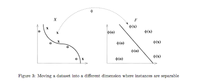
In many situations classes are not separable by a linear boundary. If this is the case, the input data can be transformed using a nonlinear mapping, φ, into another dimension space. In this new mapping, a linear boundary can be found.
When mapping into a higher dimension space, the computational complexity of the algorithm increases. Because the training process iterates through all instances as it is building its model in order to update the weights for the model, a large number of operations need to be made. It turns out that calculation of the dot product between all instances can be calculated in the lower-dimension space by substituting a kernel function into the equation. The choice of which kernel to use is experimenter-chosen, and the choice can affect the results significantly (Burges 1998).

The combination of the so-called kernel trick and the use of support vectors makes SVMs more efficient than regular linear models.

5 Applications

SVMs have been successfully used in classification problems consisting of two or many classes.
Boser, Guyon, and Vapnik (1992) evaluated SVMs for recognising hand-written digits. SVMs have also
been successfully used to classify documents by topic, and the a/b classification of images.
In the music information retrieval area, SVMs are popular for classifying audio features into a set of classes. Mandel and Ellis (2005) use SVMs for performer classification. The technique has also been used to
calculate the mood and style of songs (Mandel, Poliner, and Ellis 2006).

Here is the video of the SVM application with Rapidminer software.

Resources

1.http://www.ncbi.nlm.nih.gov/pubmed/15130823
2.http://www.music.mcgill.ca/~alastair/621/porter11svm-summary.pdf
3.https://www.youtube.com/watch?v=VVQdehQzIOU

Using Loop Operator to process multiple input resources in RapidMiner

Sometimes you may have to import the data from multiple resources into your RapidMiner model. One simple way is to import all files one by one to your model and then process them together, but this method becomes very tedious when you have to import more than 10 or 20 files. RapidMiner provides some useful operators which asset you to perform this operation automatically. In this post, I am going to share you two methods that I found to import data from multiple Excel files to the RapidMiner.

2-Simple method:

This method helps you in the case that a few numbers of resources should be imported into the model. The first step is to import all files to the model, manually. This process can be done by using appropriate “Read” Operators. In the Operators window go to the Import and then Data folders. You will see various operators are available to import different types of data into the model. In this example, I created 4 different Excel files; each contains a single row which is name and last name. As indicated in figure 1, these files can be imported to the model by “Read Excel” operators. One should notice that when this operator is used in the model, no changes in the corresponding Excel file can be made as long as the model is open. 

Figure 1

Now, in Operators window look for Append operator. This operator gets various files as input, merges them together and generates a single output table which contains all input tables. Connect all Read Excel operators to the Append operator as illustrated in figure 2.

Figure 2

Figure 3 represents the result of running this model. Each row of the output table corresponds to one input file. Since in this example, the 4 input files just consist of a single row of a name and family, for sake of simplicity, the out output consists of 4 rows.

Figure 3

2-Advanced method

Now, consider a situation that more than 10 input files should be imported into the model. In this case, the above method becomes a tedious method which requires spending tremendous amount of time to import the data manually and even gets worse whenever you want to modify the input resources. RapidMinear provides us a handy tool to perform this process easily.

 Create a new project and then in the operators windows look for Loop operators. There are various loop operators available under Loop folder in the Process Control folder. These Loop operators are used when we need to repeat certain process for a predetermined or undetermined number of iterations. Loop Files operator is the best choice for our problem. It iterates its inner operators for a set of input files in its directory. So, add it to the model and in its properties window in the Directory box specify the location of the folder contains the input files. If your input files are not in the same folder, you should remove them to the same folder. As illustrated in figure **, make sure that Iterate over files checkbox is checked.

Figure 4

Now, double click on the operator icon in the process windows to enter to the Nested process window. Then add one Read Excel operator to the Nested process window. Make sure that fil port of the process windows is connected to the fil port of the operator and its out port is connected to the out port of the process.

Figure 5

Now, use the Up arrow to back to the main process window and then add an Append operator to the model. Your model should looks like figure 6.

Figure 6